Neural networks that incorporate BayesForge to predict probabilities of binary outcomes.
General Principles
To model complex, non-linear boundaries between classes, we can extend the Bayesian Neural Network (BNN) architecture to classification tasks. While a regression BNN outputs a continuous value modeled with a Normal likelihood, a classification BNN outputs probabilities.
For binary classification, the final layer of the network condenses the hidden representations into a single output score. This score is then passed through a sigmoid activation (or used directly as the logits parameter) to map it to a probability between 0 and 1. We then use a Bernoulli or Binomial distribution to model the likelihood of the observed binary outcomes.
Considerations
Note
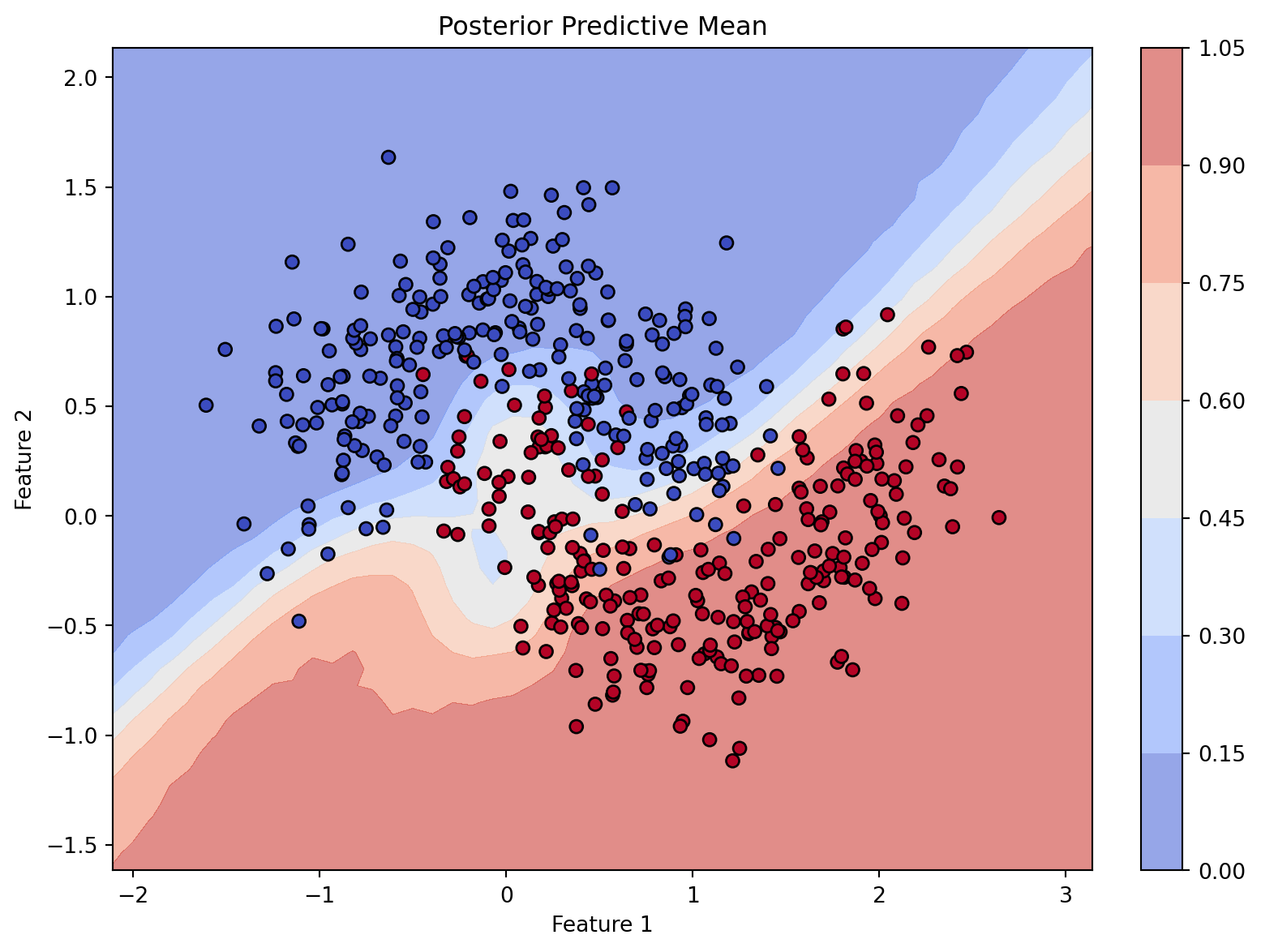
Uncertainty in Classification: In standard neural networks, softmax or sigmoid outputs are often overconfident. By using a BNN, we obtain a posterior predictive distribution that reflects true uncertainty, leading to better-calibrated probabilities. Areas with little training data will appropriately show high uncertainty rather than confident misclassifications.
Activation and Likelihood: For binary classification, we pair the linear output of the network’s final layer with a Binomial or Bernoulli likelihood. The final linear output acts as the logit input to the likelihood function, effectively applying a link function 🛈 to constrain outputs to [0, 1].
Prior distributions: Similar to regression BNNs, we apply weakly-informative priors (like Normal(0, 1)) to the weights of each layer.
Example
Below is an example code snippet demonstrating a Bayesian Neural Network for classification using the BayesForge (BF) package. This example is inspired by stochastic variational inference tutorials and uses a synthetic nested moons dataset (typically generated via make_moons).
from BayesForge import bfimport jax.numpy as jnpfrom sklearn.datasets import make_moons# Setup device------------------------------------------------m = bf(platform='cpu')# Generate Synthetic Data ------------------------------------# Two interleaving half-moon shapesX, Y = make_moons(n_samples=500, noise=0.25, random_state=42)# Convert to JAX arraysX = jnp.array(X) Y = jnp.array(Y) m.data_on_model =dict(X=X, Y=Y)# Define model ------------------------------------------------def model(X, Y, D_H1=4, D_H2=3): N, D_X = X.shape# First hidden layer: 2 input features -> 4 hidden units w1 = m.bnn.layer_linear( X, dist=m.dist.normal(0, 1, name='w1', shape=(D_X, D_H1)), activation='tanh' )# Second hidden layer: 4 hidden units -> 3 hidden units w2 = m.bnn.layer_linear( X=w1, dist=m.dist.normal(0, 1, name='w2', shape=(D_H1, D_H2)), activation='tanh' )# Final output layer: 3 hidden units -> 1 output w3 = m.bnn.layer_linear( X=w2, dist=m.dist.normal(0, 1, name='w3', shape=(D_H2, 1)) )# Squeeze the final output to match Y's shape of (N,) logits = w3.squeeze(-1)# Likelihood mapping the logits to binary outcomes m.dist.binomial(total_count=1, logits=logits, obs=Y, name='Y')# Run mcmc ------------------------------------------------m.fit(model, progress_bar=False) # Approximate posterior distributions# Predictions from the model ------------------------------------------------import matplotlib.pyplot as plt# Create a grid to evaluate the modeln_grid =50x0 = jnp.linspace(X[:, 0].min() -0.5, X[:, 0].max() +0.5, n_grid)x1 = jnp.linspace(X[:, 1].min() -0.5, X[:, 1].max() +0.5, n_grid)xx0, xx1 = jnp.meshgrid(x0, x1)X_grid = jnp.c_[xx0.ravel(), xx1.ravel()]# Swap data on model temporarily to predict on the gridm.data_on_model =dict(X=X_grid, Y=jnp.zeros(X_grid.shape[0]))pred = m.sample(samples=500)['Y']p_mean = jnp.mean(pred, axis=0)# Plotting the posterior predictive meanfig, ax = plt.subplots(figsize=(8, 6), constrained_layout=True)contour = ax.contourf(xx0, xx1, p_mean.reshape(n_grid, n_grid), cmap="coolwarm", alpha=0.6)scatter = ax.scatter(X[:, 0], X[:, 1], c=Y, cmap="coolwarm", edgecolors='k')ax.set(title="Posterior Predictive Mean", xlabel="Feature 1", ylabel="Feature 2")fig.colorbar(contour, ax=ax)
/home/sosa/work/3.12venv/lib/python3.10/site-packages/tqdm/auto.py:21: TqdmWarning:

IProgress not found. Please update jupyter and ipywidgets. See https://ipywidgets.readthedocs.io/en/stable/user_install.html
bf v 0.0.48 package loaded
jax.local_device_count 32
⚠️This function is still in development. Use it with caution. ⚠️
⚠️This function is still in development. Use it with caution. ⚠️
⚠️This function is still in development. Use it with caution. ⚠️
⚠️This function is still in development. Use it with caution. ⚠️
⚠️This function is still in development. Use it with caution. ⚠️
⚠️This function is still in development. Use it with caution. ⚠️
⚠️This function is still in development. Use it with caution. ⚠️
⚠️This function is still in development. Use it with caution. ⚠️
⚠️This function is still in development. Use it with caution. ⚠️
/home/sosa/work/BF/BayesForge/Main/main.py:674: UserWarning:

Sample's batch dimension size 4000 is different from the provided 500 num_samples argument. Defaulting to 4000.
⚠️This function is still in development. Use it with caution. ⚠️
⚠️This function is still in development. Use it with caution. ⚠️
⚠️This function is still in development. Use it with caution. ⚠️
usingBayesForgeusingPyCall# Setup device------------------------------------------------m =importBF(platform="cpu")# Generate Synthetic Data using Python's scikit-learn ---------sk_datasets =pyimport("sklearn.datasets")X = sk_datasets.make_moons(n_samples=500, noise=0.25, random_state=42)[1]Y = sk_datasets.make_moons(n_samples=500, noise=0.25, random_state=42)[2]m.data_on_model["X"] = Xm.data_on_model["Y"] = Y# Define model ------------------------------------------------@BFfunctionmodel(X, Y) N, D_X =size(X) D_H1 =4 D_H2 =3# First hidden layer w1 = m.bnn.layer_linear( X, dist=m.dist.normal(0, 1, name="w1", shape=(D_X, D_H1)), activation="tanh" )# Second hidden layer w2 = m.bnn.layer_linear( w1, dist=m.dist.normal(0, 1, name="w2", shape=(D_H1, D_H2)), activation="tanh" )# Final output layer w3 = m.bnn.layer_linear( w2, dist=m.dist.normal(0, 1, name="w3", shape=(D_H2, 1)) )# Extract logits logits = w3[:, 1]# Likelihood mapping the logits to binary outcomes m.dist.binomial(total_count=1, logits=logits, obs=Y, name="Y")end# Run mcmc ------------------------------------------------m.fit(model, num_samples=500, progress_bar=false)
Mathematical Details
In the Bayesian formulation, we place priors 🛈 on all weights and biases and define a likelihood for the output. For a classification task with a K-hidden-layer BNN with J neurons per hidden layer and a D_X-vector of predictors we can run the model as below. For the code example, we consider two hidden layers with a hyperbolic tangent (\tanh) activation function 🛈, mapped to a logit output. Because the input matrix X incorporates the intercept as its first column, the bias term is implicitly included in the layer’s weights:
Y_i is the observed binary outcome for the i-th observation.
p_i is the predicted probability of the outcome being 1 for the i-th observation.
X_i is the input row vector for the i-th observation, containing the intercept and the predictor variables. It has length D_X = 2.
H_{i,1} is the first hidden layer representation vector for the i-th observation. It has length D_{H1} = 4.
H_{i,2} is the second hidden layer representation vector for the i-th observation. It has length D_{H2} = 3.
W_1 is the weight matrix of the first hidden layer, with a shape of D_X \times D_{H1} (i.e., 2 \times 4).
W_2 is the weight matrix of the second hidden layer, with a shape of D_{H1} \times D_{H2} (i.e., 4 \times 3).
W_3 is the final layer weight matrix used to compute the logits, with a shape of D_{H2} \times 1 (i.e., 3 \times 1).
All elements within the weight matrices W_1, W_2, and W_3 are assigned independent standard Normal priors.
Notes
Note
Using m.dist.binomial(total_count=1) alongside logit inputs is equivalent to specifying a standard binary cross-entropy loss with a sigmoid activation function in deep learning frameworks.
The tutorial uses Stochastic Variational Inference (SVI) since exact MCMC approaches struggle with high-dimensional highly-correlated posterior spaces typical to neural networks. If you find MCMC chains not mixing during m.fit(), consider switching to an SVI backend or modifying priors to enforce further regularization.